2018 RFC Final Report

Analysis and editing contributions: Dan TerAvest PhD, Kristian Omland PhD (Mergus Analytics)
Data collectors, RFC survey 2018: Kris McCue, Kristian Omland, Faith Reeves, Doug DeCandia, Aaron Stoltzfus, Ellen Best, Anna Bahle, Sam Walker, and others.
RFC survey 2018 financial support: Bionutrient Food Association and donor network
RFC survey 2018 technical and moral support: Dan Kittredge, Dave Forster, Jill Clapperton PhD
Assembled by: Greg Austic

Summary

This report describes the outcomes of the 2018 Real Food Campaign’s survey of food and soil across the North East and Midwest United States. This survey was conducted from June 2018 to November 2018, with on-the-ground sample collectors (“Data Partners”) in 7 states collecting samples from 50 unique stores and 68 farms/gardeners. Two types of produce were collected, carrots (648 total samples) and spinach (181 total samples), with 0-6’’ and 6-12’’ soils sampled when collecting from the field (177 samples at both 0 – 6’’ and 6 – 12’’ depths).

The objectives of this year’s survey were 1) to determine the spectrum of variation in food quality and soil quality from a reasonably representative sampling of our food supply, 2) to identify relationships between farm practice, soil quality, and food quality in the data, and 3) to attempt to predict, using spectral data and metadata, nutritional parameters in the produce. Broadly, the outcomes were:

• There is significant variation (up to 200:1) in antioxidants, polyphenols, and minerals in carrots and spinach from a variety of sources (farms, farmers markets, stores).

• There was significant variation in quality due to brands and farms, but no meaningful variation between the basic farm management questions asked in the survey. This is possibly due to too little data, overly general farm practice information, or no connection with the survey questions asked. Finally, a large portion of the variation in quality could not be determined given the information collected.

• Spectral reflectance data from carrot and spinach extracts correctly identified high (>50th percentile) versus low (<50th percentile) polyphenols and antioxidant samples 73 – 86% of the time. Reflectance data from surface scans were only 61 – 74% accurate. Spectral data, especially those in the UV range, were important predictive variables in the models. Both linear regression and random forest models were used.

Background

The Real Food Campaign (RFC) emerged in 2018 from a partnership between the Bionutrient Food Association (BFA) and its membership, Next7, Our Sci LLC, farmOS, and others.  The mission of the RFC is to identify the best ways to drive increased nutrient density in our food supply, specifically through a better understanding of soil health, food quality, human health and their connections.  For the full description of RFC mission, goals and objectives go here.

RFC’s goals in 2018 are two fold: 1) to better understand the  variation in food nutrient density in the food supply, and identify possible sources of variation that relate to soil health and farm practice, and 2) to attempt to correlate spectral reflectance of produce with standard lab nutritional measurements like antioxidants, polyphenols, proteins, various minerals, etc.

The 2018 season will end in November, and final results are expected by end of December 2018.  This report is an in-process update for donors, BFA members, and the general public.

Overview of activities

The following activities and milestones were accomplished in  2018:

• A survey was designed to collect farm and market data from the NE and MW US, and soil and food testing methods were chosen to quantify food quality and soil health

• The Data Partner program was created with 7 collaborators who signed on to submit 6 – 18 samples to the lab per week

• A lab location was identified, equipped and staffed in Ann Arbor MI to measure soil quality and food quality

• An lab sampling/testing process was created and optimized throughout the summer

• A scalable, open source information management system was developed specifically for use within the lab, and plans laid for integration with other systems (like FarmOS) to collect more detailed farm-level data (source at gitlab)

• A handheld reflectometer (bionutient meter) was designed, tested, built, and used daily in the lab (source at gitlab)

• 829 carrot, spinach, and soil samples were processed from stores, farms, and farmers markets in 6 states from 7 data partners

Methods

Link to description of survey concept and methodology https://lab.realfoodcampaign.org/survey/. This includes links to the testing methods for soil and food samples.

Once completed, the data required some clean-up. Typical issues which caused data errors or inconsistency were:

• Errors were made early in the season while the lab finalized its internal methods for antioxidants, polyphenols, etc.

• Some samples were delayed in the mail, making them rotten by the time they reached the lab.

• Some sample vegetables were too small to test.

• Metadata surveys were either not submitted via the web or were not completely filled out, resulting in some missing metadata..

• Samples from the same farm or store were not marked the same every time (like “sam’s farm” versus “sams farm” versus “sam’s farm store” etc.) and dates were manually inputted using different formats (11/6/2018 versus Nov 6, 2018 etc.)

As much analysis as possible was done in Javascript and is publicly available. The data available on the web is mostly cleaned for the aforementioned errors except for date and time inconsistencies. The full analysis and visualization, and cleaned download link (csv format) is available here https://app.our-sci.net/#/dashboard/by-dashboard-id/bfa-v2.  There are full links to all web-based analysis, visualizations, and access to the raw data in the “Describing the Variation” section below.

The remaining minor changes for date/time were completed in LibreOffice Calc, and that result is not available publicly because it contains farm-level details. If you are interested in that data, please contact us directly at lab@realfoodcampaign.org and we can provide it.

Describing the Variation

Summary

There was wide variation in many of the measured values across soil, carrots, and spinach. Some examples include soil respiration (from ~0 to ~50 micrograms of mineralizable carbon per gram of soil), total organic carbon (from ~0 – ~13% dry weight carbon), antioxidants in carrots (~0 – ~250) and spinach (~50 – ~1000), and minerals in foods like Potassium (~5000 – ~90,000) in carrots or Iron (~50 – ~1400) in spinach. However, the sources of this variation due to farm practice were not clear from the existing data, possibly due to too little data, overly general farm practice information, or no connection with the survey questions asked. Variation was measured within a bag or a field of carrots (coefficients of variation between 5% – 32%) as well as between brands or farms (coefficients of variation between 35.5% – 61.8%). Therefore, given the clear variation relating to differences in brand, farm and time of year, it would be worth further investigating variety and development stage as likely causes of the variation.

Details

A quick note on terminology… We are going to use the term “meaningful” below to describe findings, like “there is not meaningful difference between A and B”. In academic papers, it would be more typical to use “statistically significant” and talk about p-values, but we feel that is often prone to errors we want to avoid especially in large observational datasets of this type. Specifically, we want to avoid identifying relationships which exist only because of random chance due to a large number of variables in the dataset, and overplaying differences which are technically statistically significant and also true but so small that they don’t indicate an outcome of importance. As such, “meaningful” is for findings which are both of reasonably high statistical significance, and reasonably high absolute difference such that the outcome matters in the real world.

For histograms and other descriptive information about the minerals analysis, see the following:

Histograms, graphs, visualizations of data

General data overview + download links (.csv)

Histograms of all minerals (food and soil)

Comparison of soil minerals between layers

Comparison of soil minerals to food minerals

Comparison of soil respiration by minerals in food

Comparison of food minerals to each other

From a visual review of the data, its clear that there is significant variation on almost every measure (minerals in soils and food, antioxidants and polyphenols, soil carbon and soil respiration).  To attempt to explain some of the variation, we pose several questions to the data and attempt to answer them.

How much variation is there within a single field, or bag of carrots, versus between fields or bags of carrots?

In general, 3 – 6 samples came from the same bag or basket (in the store or farmers market) or same field (from a farm).  To identify the variation within a field or bag, the data was grouped by date/time collected and county, with groups of less than 3 samples removed because standard deviation cannot be reliably calculated.  The mean and standard deviation was calculated for the total population, and then for the groups, to see if the data became more clustered (lower standard deviation) when looking only at the groups.  When available, estimates of lab variation were added as well.

This is a very rough way of estimating the source of noise – the coefficient of variation (mean divided by standard deviation) is only one way to understand how clustered a population is.  So any given value should be taken with a grain of salt. However, it provides a coarse look at this particular, limited data set.

Table 1: Summary Statistics and Sources of variation in Antioxidants and Polyphenols

Table 2: Summary Statistics and Sources of variation, Minerals

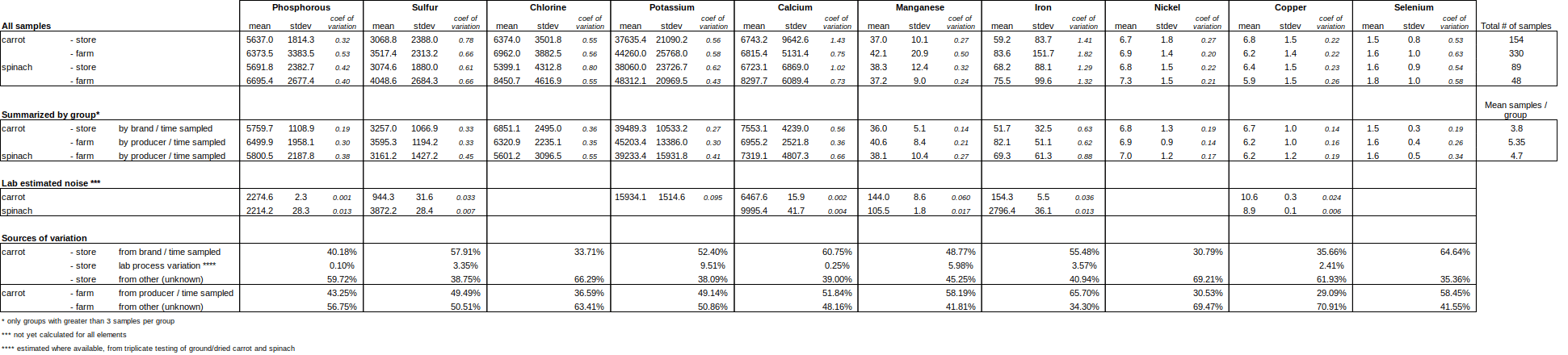
While the average values do not differ much between farm and store, the source of variation does.  The brand of carrot and time sampled groups accounts for only 26-30% of the variation among the store bought samples, while the producer and time sampled groups accounts for 48-60% of the variation in farm collected samples for antioxidants and polyphenols.  This is due to the fact that farm collected samples tend to have higher variability as a group and lower variability within the farm / time sampled group.  This does not hold true for minerals, where farms or stores may be more variable depending on the mineral.

In all, there are no meaningful differences in average values between farm or store collected samples, but it is worth noting that certain parameters are highly variable, while others are very stable.  For example in carrots, Iron and Calcium is highly variable (coefficient of variations between 0.75-1.82), while Copper, Nickel, and Manganese do not very much at all (coefficient of variations between 0.22 – 0.5).  While we do not have a perfect understanding of our in-lab sources of error, the repeatability tests we have run on minerals show pretty low noise due to the measurement instrument (XRF) and sample prep error, so the minerals data is probably pretty accurate.  The antioxidants and polyphenols are benchtop methods measuring oxidation and pH changes and probably have higher sources of variation due to lab process and sample prep.

Another way to look at this is to identify side-by-side comparable groups 3 or more samples from the same location, brand, field, at different time points.  Its important to note that calculating a standard deviation from small groups (3 – 6 samples) will not be very accurate on a group by group basis.  As such, this is less quantitative and more qualitative (ie one step above reading tea leaves), but it can be helpful to identify and understand outliers.  A set of such groups were pulled from the data, the mean and standard deviation was calculated for the total population, and then for the groups, to see if the data became more clustered (lower standard deviation) when looking only at the groups.

Table 3: Antioxidants and Polyphenols.  Comparable groups at different time points based on brand / location for stores, or farm for farms. Varietal information is referenced for farm samples if known.  Notable data points are bolded.

Table 4: Minerals. Comparable groups at different time points based on brand / location for stores, or farm for farms. Varietal information is referenced for farm samples if known. Notable data points are bolded.



Notable items from these tables:

• In Table 3, Collected on Farm section: The comparison of Deep Purple and Jaune Du Daubs (white) varieties shows the clear effect of color – antioxidants and polyphenols are very different between the two.

• The same grower or brand can have very different results when sampled at two different periods. Note in Table 3 “Hartford, Kern Ridge” and “Hannafords” samples. This is also true for minerals, in Table 4 note “Jefferson, variety Danver” for Phosphorous, Chlorine, Potassium, and Calcium. In this case, even the variety was shown to be the same. Also note in Table 3 the “Fairfield…” and “Hartford…” and “Grimmway…” samples with variation in Sulfur, Chlorine, Calcium, Potassium, and Iron.

• Most elements have very normal distributions. However, there are some elements which have normal distributions with one or two extreme outliers. Calcium (Table 4, “Washtenaw…” groups and “Kern Ridge…” group) and Iron (Table 4, “Fairfield…”, “Westchester…”, “Lenawee…” groups).

Does the variation follow expected patterns?  For example, do polyphenols and antioxidants tend to vary together?  Do total carbon/soil respiration/minerals in top soil versus bottom soil correlate?

Overall, the relationships that we would expect between soil layers (high carbon and minerals in 0-6’’ → high carbon and minerals in 6 – 12’’ soil), between soil carbon and soil respiration (high carbon → high respiration)  and between antioxidants and polyphenols (high antioxidants → high polyphenols) in food samples hold true. This provides some baseline sanity check that the methods used to measure food and soil were at least somewhat accurate.  See below graphs for examples.

Is there a relationship between food nutrition and farm practice?

There is no obvious correlation between farm practice and food nutrition based on the very limited farm practice data collected this year.

The following categories were created to identify differences between more or less regenerative practices.

There are no meaningful (large and/or statistically significant) differences between these categories.  The graphs below shows averages between the categories across antioxidants, polyphenols, proteins, and various minerals.

While there are some differences, none are meaningful with the possible exception of the iron levels in farm-only samples.

Is there a relationship between soil biological activity and food nutrition? 

Based on the current data, there is no obvious relationship between the relatively simple measurement of soil biological activity and any of the food quality measures.  Simple XY graphs show no obvious trends either by antioxidants, polyphenols, or minerals (as examples, antioxidants by soil respiration and potassium by soil respiration shown below).

Predicting nutritional content

Summary

Using two models, prediction of carrot and spinach quality (antioxidants and polyphenols) ranged from roughly 60 – 80%, depending on the model, produce type, and variables included.  While several wavelengths of the spectral data improved model fit, data in the UV range showed the largest improvement in model fit for antioxidants and polyphenols in carrots.

Details

Two types of models (random forest, linear regression) were used to correlate antioxidants and polyphenols with spectral data and some metadata.  Each has benefits in certain situations, two were used here to reduce the likelihood of model overfitting and improve the likelihood of avoiding statistical artefacts.

Random Forest

The random forest model was tested with spectral data from the Bionutrient Meter Beta only (10 wavelengths from 365nm to 940nm), some metadata (carrot diameter, state collected in, week of the year it was collected, and visually identified carrot color), and an optimized version with the top 10 highest impacting variables on the model.  Both the surface and supernatant (methanol/water extraction + centrifuge) were scanned and modeled separately.

As a control, metadata only models (no spectral data) were also performed for comparison (not shown).  Results were poor, ranging from 53 – 57% correct, indicating that spectral data significantly improved the model fit.

The results are shown in the tables below for carrots and spinach, respectively.

Several of the spinach samples were known to not technically be spinach.  These varieties also clearly contributed to some outlier values in the data, as compared to other typical values.  The list of these values is:

The model for spinach was re-run with these samples removed.  Results shown in the table below.

Variables of importance

The most important predictive variables are shown below for the optimized carrot model for polyphenols (both surface scan, and supernatant scan).  Mean-square error (MSE) describes the effect of the variable being randomly shuffled on the model MSE. An increase indicates that the model quality went down as a result of this shuffling.  In this case, the higher the number, the more important the number in the prediction.

nmXXX – the Bionutrient Meter value at a given wavelength (365, 385, 450, …)

Weeks – the week of the year that the sample was collected (0 – 52)

STATE – the state the sample was collected in

Carrot color – external color of the carrot (orange, purple, red, white, other)

diameter – diameter of the carrot near the top in cm

In both graphs, models fitting data from supernatant scans are in blue and raw surface scans are in orange.

Impact of data quantity of model fit

The model used for carrots was re-run (re-trained) with varying numbers of samples from 107 to 320, to determine if the r2 continues to improve with more training data.  The graphs below show a better fit as the number of samples in the training set increases. While at some point the model will not improve with more data, it is clear that at least up to 320 samples shows continued improvement of the model fit.

Impact of data quantity on model fit

Linear Regression

Linear regression with automated variable selection was also used to try to predict nutritional quality based on spectral data.    In this case, principal component analysis was used to generate a total score between polyphenols and antioxidants. For carrot surface scans, results were similar to above, with a combined 29 + 34 = 63% predicted correctly, compare to 62.2% and 76.3% using random forest.

Model selection supported including terms representing biological amendments and cover crops but each had a negative coefficient (lower antioxidants/polyphenols with amendments or cover crops) so that model was not used for prediction; inclusion of organic practices and irrigation was not supported. In imitation of the random forest model described above, models including week, state, and carrot diameter were considered (all carrots in this analysis were orange, so effect of color was not modeled). Results from week 29 (unusually high readings) and week 31 (unusually low readings) were unusual and model fitting was susceptible to being dominated by those readings. A random effects model fit to the data from week 32 on showed that week accounted for less than 0.3% of the variation in the data. Among the three well-represented states, there was substantial variation attributable to state (positive for CT, neutral for MI, and negative for NY); however, inclusion of random effects is not available in the automated model selection routine and manual model selection was prohibitive.

Carrot quality was positively related to carrot diameter in the data set and inclusion of diameter as a covariate permitted adjusted R-squared to improve from 0.201 to 0.225 for direct scans and from 0.418 to 0.488 for extracts. However, diameter was not added to the simulations based on scans alone.

The same method using carrots only but measuring the supernatant rather than the surface, achieved 36 + 38 = 74% predicted correctly compared to 72.1% and 73.2% using random forest.

Lessons learned, next steps

We learned a huge number of small lessons in creating the lab, in terms of process improvements and optimization, as well as some larger overall lessons.  These larger lessons are described below, with next steps planned in 2019 noted in italics.

We need more quality, granularity, and quantity of data

The farm practice information was extremely spotty and not very descriptive of the actual farm.  It is clear we need to focus on identifying variety and planting / harvest date as they are likely two major drivers of variation we saw this year.  In addition, the prediction models showed that 300 – 400 data points was too few, and more would produce a better model (up to a point of course).  Finally, we didn’t nail down the noise caused by our lab method itself, which made it hard to see the effects through what may have just been lab noise.

<– We are currently nailing down our lab process to both quantity noise and reduce it.  Also, we’ve initiated the farm partners program to collect weekly farm practice data (granular), in addition to the data partners program who’ll be collecting from stores and farmers markets.  All partners will be collect data via phone, which will reduce lab time and increase information about the farm (like weather and soil data).  Finally, we targeted 800 – 1000 samples per crop this year, and expanded the crops to make Data Partner’s collection efforts more fruitful (har de har har). 

The survey produces more data than one person can analyze

In writing this report it became clear that we didn’t have all the knowledge in-house to look at this data.  A good example are the suite of interesting graphs relating minerals to each other in food, with very strong correlations between silicon and aluminum, nickel and copper, and many other things.  Also, there were interesting outliers among the farms and stores that deserve a second look.  We hope that the BFA community has a chance to dive into this report and share thoughts and insights.

Identifying good, consistent Data Partners is essential to our success

Collecting samples from a wide range of locations over time is a key part of what makes the RFC effective and inexpensive.  Sample collection, even when very simplified, does take both time and some experience to do correctly.  We found that individuals sending a few samples was time consuming for the lab, produced low quality samples, and was frustrating for the individuals.

Also, not everyone is cut out to be a Data Partner.  It requires visiting farms and stores every week, consistently and paying attention to detail.  We learned from feedback that 2 – 3 sampling locations per week was probably too much, even for the committed and amazing volunteers we had in 2018.

In the future, we should expect that for every 2 people we sign up for the Data Partners program, we get 1 to stick around and send quality samples throughout the season.

<– This year we are reducing the expectation for a data partner to just 1 sampling location per week.  In addition, due to the Farm Partners program which will increase on farm-direct samples, we can reduce the Data Partners farm-direct sampling which was the most time consuming ask.

Shipping is not easy, cheap, or without error

Early  in the season several samples were lost or delayed in shipping, even using the higher level (USPS Priority Express) service.

We also were told that we should get a USPS corporate account, which would save us money on shipping, and allow us to print our own labels (you cannot print USPS Priority Express labels using a normal account).  We will pursue this for 2019.

Overall, our shipping issues have been addressed, but caused lots of headaches early on.

We need to fix (no more changes!) our testing methodology by early spring

Once a sample arrives in the lab, it goes through a long and detailed set of procedures which must be done consistently to be confident that data is comparable over time.  We had to change procedures several times this year to address problems with our testing methods and to improve efficiency.  Every time a procedure or test changes its version, it causes a lot of headache when analyzing the data, and calls into question comparability of samples over time, effectively reducing the power of the data.

We should minimize these in-season changes in future years and spend the winter creating a process we are confident in as soon as the survey begins in the spring.

<– We have connected with Selena Ahmed’s lab at UM to improve our lab process and have partnered with Cyndi Daily at Chico State to build another full sampling lab on the west coast.  The west coast RFC lab will target 800 – 1000 samples in 2019 and expand the number of states we can take samples from.  We have also connected with our Farm and Data partners months ahead, so hopefully we’ll be more on time this year.

Committed lab staff (full time, living wage) are essential to our success

Initially, we hired a 3/4 time lab manager to process samples, write out procedures, and help us improve the lab process.  While this person was good and in fact enjoyed the job, she changed jobs after 3 months because she needed more full time and long term work.

In order to bring professionalism and consistency to the lab, we need a full time position which has at least 6 months of funding.  Retraining lab personnel is time consuming, causes errors and/or inconsistency in the data, and puts us in a position of reworking old ground rather than making our process better in the future.

We are also looking into internships, credit hours, and collaborations with university labs at U of M to support this full time person with student hours.  We hope that students also benefit from learning about the RFC and being inspired by its mission.

<– we have pulled in 2 part time students, 1 student may come on full time as she graduates, hired a full time lab manager and full time lab tech.  We are also beginning to get interest in the RFC Lab Residency we offer, with our first expected residency sometime in July.

Expenses

Below are actual and project expenses for the RFC Lab in 2018.
Detailed report of contract software, hardware, and consumables (excluding XRF, includes part lab labor but not all) here.

Projected cost per sample in 2018 ($212.85), is about half of a quoted commercial alternative for a similar suite of tests, and includes all costs including software, hardware, and equipment.

The projected cost per sample for 2019 (116.95 – 60.04 per sample), which removes the up-front costs associated with the XRF and hardware/software and assumes some efficiency gain, is a more realistic long-term range for per-test cost.